Methodological Details
Participants
Participants were drawn from the Studying Adolescents in Realtime (STAR) study dataset. The STAR study is a massive ongoing data collection effort organized by Dr. Katie McLaughlin, designed to examine the mechanisms linking early life stress to psychopathology. All subjects were recruited from the greater Boston area and were selected to have variability in race, ethnicity, and socioeconomic status. The final analytic sample used in the projects here consists of 30 subjects ages 13-17, assessed monthly over the course of a year. Each subject completed 12 monthly visits consisting of a life stress interview, surveys to assess mental health and social behavior, behavioral tasks, and a 60-minute MRI scan session that included the canonical emotion processing task, as well as a resting-state scan (aka. the fixation task).
Measures Description
Stressful Life Events:
The UCLA life stress interview was used to document stressful life events and was administered during each monthly session (Hammen, 1988). The UCLA life stress interview is a semi-structured interview that objectively assess for acute life events (aka. episodic stressors) such as failing a test or the break-up of a romantic relationship, as well as chronic stress such as long-term medical challenges. The interview involves a series of structured prompts that query an extensive set of domains in which an individual may experience either acute or chronic stress including peers, parents, household/extended family, neighborhood, school, academic, health, finance, and discrimination. If a participant reports a stressor, the timing, duration, severity, and coping resources available are additionally recorded. The severity of each reported acute/chronic event is objectively coded by research personal using a 9-point scale (including half points), ranging from 1 (none) to 5 (extremely severe). The UCLA interview employed was adapted for use in adolescence and has been well validated (Daley et al., 1997; Dohrenwend, 2006; Hammen, 1991). For the purposes of this work, we will focus on the acute stress (aka. episodic stressors) component of the UCLA. An overall episodic stress score was calculated by summing the severity scores of all reported events for the given month, capturing both the quantity and intensity of episodic stressors (Hammen et al., 2000). These epsodic stress scores will be referred to as stressful life events for the remainder of this work. Participants received a score of zero if no stressful life events were documented. The interview was administered at each monthly visit to assess stressful life events occurring since the previous visit.
Psychopathology Measures:
Depression Symptoms: Depression symptoms were evaluated during each study visit using the Patient Health Questionnaire-9 (PHQ-9) scale, which measures symptoms experienced over the preceding two weeks. The scale consists of nine items, each rated on a Likert scale from 0 to 3, with higher scores reflecting more severe symptoms. The PHQ-9 is recognized for its reliability and validity, as reported by Kroenke et al. (2001).
Anxiety Symptoms: Generalized anxiety symptoms were assessed at each study visit using the Generalized Anxiety Disorder-7 (GAD-7) scale, which evaluates symptoms from the past two weeks. This scale comprises seven items, each rated on a Likert scale from 0 to 3, where higher scores indicate greater severity of symptoms. The GAD-7 has good reliability and validity, as reported by Spitzer et al. (2006).
fMRI Data Aquisition and Preprocessing:
Mock Scanner Training.
Prior to the first scan session, participants were oriented with the sights and sounds of the MRI machine using a mock scanner a technique known to improve image quality in more difficult to scan populations (de Bie et al., 2010). Participants practiced lying still as they watched a movie after being placed inside the mock-scanner bore. The movie would pause if head motion exceeded (starting at 0.5 and reducing down to 0.1).
MRI Data Acquisition
All scans were collected at the Harvard Center for Brain Science, using a 3T Siemens Magnetom Prismafit MRI scanner and 32-channel head coil (Siemens Healthcare, Erlangen, Germany). Foam pads and/or pillows were used to help with head immobilization and participant comfort. Participants viewed movie or stimuli for task-based functional scans through a mirror attached to the head coil. At the beginning of each scan session, the viewing location was confirmed to be in the center of the field of view and at a comfortable angle for viewing. During each scan session, rapid structural (T1/T2-weighted) images, fixation- and task-based functional (T2*-weighted) images, and diffusion-weighted images were acquired (full imaging protocol details can be found in Table 1).
Rapid T1w images were acquired using a 1.2 mm Multi-Echo Magnetization-Prepared Rapid Acquisition Gradient Echo (MEMPRAGE) sequence with the following parameters: TR = 2200 ms, TE = 1.5/3.4/5.2/7.0 ms, TI = 1100ms, Flip Angle = 7o, Matrix 192 x 192 x 144, in-plane generalized auto-calibrating partial parallel acquisition (GRAPPA) acceleration =4, and Scan Length= 2:23 mins (van der Kouwe, Benner, Salat, & Fischl, 2008). T2w images were acquired using a 1.2mm isotropic single-echo sequence with the following parameters: TR = 2800 ms, TE = 326 ms, Variable Flip Angle, Matrix 192 x 192 x 144, GRAPPA acceleration = 2, and Scan Length= 2:37 mins. The first and last scan sessions also included a set of T1w and T2w images acquired with the Adolescent Brain Cognitive Development (ABCD) study imaging protocol (Casey et al., 2018), increasing the length of these scan sessions by 30 minutes. T1w images were acquired with the following parameters: TR = 2500 ms, TE = 2.9 ms, TI = 1070ms, Flip Angle = 8o, Matrix 256 x 256 x 176, GRAPPA acceleration = 2, and Scan Length= 7:12 mins. And the T2w image with the following parameters: TR = 3200 ms, TE = 565 ms, Variable Flip Angle, Matrix 256 x 256 x 176, GRAPPA acceleration =2, and Scan Length= 6:35 mins. All structural image protocols included embedded volumetric navigators (vNAV) that were used to track changes in head position during acquisition (Tisdall et al., 2016).
functional MRI data was acquired with blood oxygenation level-dependent (BOLD) contrast (Ogawa, Lee, Kay, & Tank, 1990) using a T2*-weighted sequence described the HCP-D protocol (Barch et al., 2013; Harms et al., 2018; Somerville et al., 2018). All BOLD runs were acquired with a multiband gradient-echo echo-planar pulse with the following parameters: voxel size = 2.0 mm, TR = 800 ms, TE= 37 ms, Flip Angle = 52 o, matrix = 208 x 208 x 72, and SMS factor = 8 and provided full coverage of cerebrum and cerebellum. Most functional tasks were acquired in both Anterior-to-Posterior (AP) and Posterior-to-Anterior (PA) phase encoding directions. However, the Emotion task and Working Memory task were acquired in PA phase encoding direction only. The first 10 volumes (TRs) of all BOLD runs were removed prior to preprocessing for T1 equilibration.
Spin-echo (AP/PA) field map pairs were acquired with the following parameters: voxel size = 2.0 mm, repetition time (TR) = 8 000 ms, TE= 66 ms, Flip Angle = 90 o, matrix = 208 x 208 x 72, and SMS factor 8, and were used to correct for spatial distortions. During most sessions, two spin-echo field map pairs were acquired. Two additional spin-echo field map pairs were acquired during the first or last scan sessions. Additional spin-echo field map pairs were acquired if the participant required a break during the scan session to match new localized and AAScout settings.
The raw DICOM images for all neuroimaging data is hosted on Extensible Neuroimaging Archive Toolkit (XNAT) (Marcus, Olsen, Ramaratnam, & Buckner, 2007) software platform. Images were then copied to local storage using ArcGet (with direct export to BIDS organization https://yaxil.readthedocs.io/en/latest/arcget.html#direct-export-to-bids-beta), and conversion from DICOM to NIFTI image type (using dcm2niix v1.0.20200331) (Li, Morgan, Ashburner, Smith, & Rorden, 2016). Automated functional quality assessment measures available through XNAT (Fariello, Petrov, O’Keefe, Coombs, & Buckner, 2012) were utilized for fMRI quality checking and participant feedback.
Data Exclusion and Quality Control
All T1w/T2w images were quantitatively and qualitatively inspected. Our T1w and T2w imaging protocols included embedded volumetric navigator (vNAV (Tisdall et al., 2016)) images; which are very rapid, low-resolution images that are simultaneously obtained during the T1w (or T2w) image acquisition then registered together to track head motion in real time. The vNAV images were processed using code available (https://github.com/harvard-nrg/vnav), and motion metrics obtained. Images were excluded if the mean motion score exceeded 10 RMS/Min, due to the influence of motion on brain estimates (Reuter et al., 2015). Images were analyzed with MRIQC toolbox (v.0.14.2) to obtain metrics of image quality including signal-to-noise, and image smoothing.
All T1w/T2w images were inspected at the scanner console for the presence of wrapping, ringing/blurring, ghosting, radio frequency noise, signal inhomogeneity and susceptibility artifacts. When present, the artifact was rated as mild, moderate, or severe and findings documented. Internal laboratory training materials for visually inspecting the data and artifact scoring rubric are included in the supplemental materials. All training examples came from the Oxford Neuroimaging Primer Series (http://www.neuroimagingprimers.org/), or the Harvard CBS Quality Control Manual (http://cbs.fas.harvard.edu/facilities/neuroimaging/investigators/mr-data-quality-control/).
Real-time motion tracking during the scan was done using Framewise Integrated Real-time MRI Monitoring (FIRMM; (Dosenbach et al., 2017)) or prototype “ScanBuddy” software; which runs FSL’s motion correct linear registration (MCFLIRT, FSL v5.0.4; (Jenkinson, Bannister, Brady, & Smith, 2002)) after the scan completes to provide estimates of absolute and motion spiking. All images were inspected at the scanner console for the presence of artifacts and findings were documented. Participants were reminded throughout the scan session to remain still during the scan. Time rarely permitted a rescan. Eye glaze was monitored and recorded during fixation BOLD runs.
BOLD runs were given a motion score out of 5 (i.e. ranging from 1-Unusable to 5-Excellent)(see Table 2), based on automated functional quality assessment measures available through XNAT (Fariello et al., 2012). To obtain a score of 5, the BOLD run could not (1) exceed 2mm of maximum absolute motion, or (2) contain 5 or more > 0.5mm motion spikes, or (3) have a slice-based signal-to-noise ratio (SNR) < 125. Motion score for all BOLD runs acquired in the previous session were given to participant as feedback at the next scan session to help encourage stillness
As a first pass, BOLD runs were excluded from preprocessing if (1) the maximum absolute motion exceed 4mm, (2) 10 or more > 0.5mm motion spikes occurred, or (3) the slice-based signal-to-noise ratio (SNR) was < 125. Runs with SNR > 100 but < 125 were included if absolute motion and spike thresholds were not exceeded. During preprocessing, BOLD runs were additionally excluded if > 20% of its volumes (TRs) exceeded Framewise Displacement (FD > 0.5mm for fixation, and > 0.9mm for task) or Derivative of rms VARiance over voxelS (DVARS > 1.5Quartile) thresholds to exclude extreme changes whole-brain signal (Power, Barnes, Snyder, Schlaggar, & Petersen, 2012; Power et al., 2011; Power et al., 2014). An outlier regressor matrix (containing all TRs that exceeded the motion threshold was included in task-based general linear models. Fixation BOLD runs included a 36-parameter model, shown to improve control of motion artifacts known to corrupt resting-state functional connectivity analyses (Satterthwaite et al., 2013) described in more detail below. BOLD runs were not excluded based on behavioral performance.
Structural processing pipeline
Structural images (T1w and T2w) images were preprocessed using similar methods to those outlined by Human Connectome Project (HCP) (Glasser et al., 2013) and Adolescent Brain Cognitive Development (ABCD) (Hagler Jr et al., 2019) study protocols. Images were corrected for MR gradient-nonlinearity induced distortions using a scanner-specific gradient coefficient file available from Siemens and gradient_unwarp package (https://github.com/Washington-University/gradunwarp) (Jovicich et al., 2006; Polimeni, Renvall, Zaretskaya, & Fischl, 2018).
Next, T1-weighted images (and T2-weighted images whenever possible) were processed using FreeSurfer v7.2.0 image analysis suite (http://surfer.nmr.mgh.harvard.edu/). The details of FreeSurfer’s automated recon-all pipeline have been described previously (Dale, Fischl, & Sereno, 1999; Bruce Fischl, Sereno, & Dale, 1999). Rapid 1.2mm isotropic MEMPRAGE images are up-sampled to 1mm isotropic resolution, non-brain tissue is removed using a hybrid watershed/surface deformation procedure (Ségonne et al., 2004), B1 bias-field correction was applied using standard correction methods (Sled, Zijdenbos, & Evans, 1998), and an automated calculation of the transformation to atlas space is performed. Next, white matter and subcortical structures including the hippocampus, amygdala, caudate and putamen were segmented (Dale et al., 1999; Bruce Fischl et al., 2002; Bruce Fischl et al., 2004). Next, additional intensity normalization (Sled et al., 1998) and tessellated mesh, consisting of ~40,000 triangular vertices per hemisphere, of the gray/white and gray/dura boundaries were defined (B Fischl & Dale, 2000; Bruce Fischl et al., 1999). Cortical thickness was calculated for each vertex as the shortest distance between these boundaries (B Fischl & Dale, 2000). Regional volumes, surface area and thickness estimates were parcellated from the standard 32 gyral-based parcellation (per hemisphere), defined from the Desikan-Killiany atlas (Desikan et al., 2006; Bruce Fischl et al., 2004). Images continued their processing through the longitudinal stream of FreeSurfer (Reuter, Schmansky, Rosas, & Fischl, 2012) for structural analyses. To do this, an unbiased subject-specific template using robust, inverse consistent registration, reducing the bias toward any single scan (Reuter, Rosas, & Fischl, 2010). Several processing steps including skull-stripping, atlas registration, surface-based registrations and parcellations are initialized from a subject-specific template, increasing the reliability and statistical power of the resulting estimates (Reuter et al., 2012). Functional preprocessing pipeline
Data were preprocessed using an in-house preprocessing pipeline (“iProc_STAR”); combining previously published methods for optimizing alignment between BOLD runs (iProc; (Braga & Buckner, 2017; Braga, Van Dijk, Polimeni, Eldaief, & Buckner, 2019)) with improved detection and removal of motion artifacts (Power et al., 2014; Satterthwaite et al., 2013) and improved registration to standard MNI space (Avants, Tustison, & Song, 2009; Tustison et al., 2014)). Pipeline decisions were informed by commonly used preprocessing toolbox fmriprep (Esteban et al., 2019), as well as HCP minimally processed pipelines (Glasser et al., 2013; Somerville et al., 2018) and by the ABCD study (Hagler Jr et al., 2019) methods, to further optimize our preprocessing pipeline for use in child and adolescent populations. All preprocessing steps were first calculated and then applied as a single interpolation to minimizing spatial blurring. Full details are described below.
BOLD data were interpolated to 1mm isotropic T1-weighted native volume space by applying 4 transformation matrices in a single processing step. The first matrix (MAT1) was used to correct for head motion. Motion parameters were calculated with respect to a middle volume using linear registration rigid body translation and rotation with 12 degrees of freedom (MCFLIRT, FSL v5.0.4; (Jenkinson et al., 2002)).The middle volume was confirmed as not a motion outlier using the FD and DVARS criteria described above. If the selected middle volume was a motion outlier, a new middle volume was chosen (± 2 TRs from the previous selection) and the motion parameters (MAT1) were recalculated with respect to the new middle volume.
The second transform matrix (MAT2) was used to correct for field inhomogeneities caused by susceptibility gradients (Jenkinson, 2004). Spin-echo field maps were used to correct for distortions in BOLD images. Field map unwarping was calculated to the BOLD run’s middle volume by first converting the spin-echo field maps to phase and magnitude images and calculating the transform matrix (using FUGUE, FSL v4.0.3; (Jenkinson, 2004; Smith et al., 2004)).
The third matrix (MAT3) was used to align each BOLD run to the within-individual mean BOLD template (12 DOF; FLIRT (Jenkinson et al., 2002)). The within-individual mean BOLD template was created by taking the average across all aligned fieldmap-unwarped middle volume images for each BOLD run, reducing bias toward any single BOLD run. To do this, first a single fieldmap-unwarped middle volume as selected as a temporary target. All fieldmap-unwarped middle volume images (for each BOLD run) were registered to this temporary target and an average taken as the within-individual mean BOLD template.
The fourth matrix (MAT4) was used to align the mean BOLD template to the structural T1w image. The mean-BOLD template was up-sampled to 1mm isotropic resolution to improve registration to the up-sampled 1mm T1w template target. Boundary-based registration algorithm from FreeSurfer, initialized with FSL (6 DOF; bbregister (Greve & Fischl, 2009)) was used to register images together. For each BOLD run, transform matrices (i.e. MAT1 through MAT4) were combined using FSL’s convertwarp tool, and applied in a single interpolation using FSL’s applywarp tool. The resulting processed BOLD runs were motion corrected (MAT1), unwarped (MAT2), between-BOLD aligned (MAT3) and projected to T1 native space (MAT4). Individual cortical surfaces were also projected to fsaverage6 atlas cortical surface space (40,962 vertices per hemisphere (Bruce Fischl et al., 1999)) from individual T1-space. Finally, surface-based estimates were smoothed using a 4mm full-width-at-half-maximum (FWHM) Gaussian kernel.
A fifth matrix (MAT5) was used to further align individual T1native space to MNI atlas space. Registration was performed using Advanced Normalization Tools (ANTS v2.4.4; 3-stage: rigid, affine and deformation syn algorithm and neighborhood cross correlation as the selected similar metric) (Avants et al., 2009). For analyses with the target of MNI atlas space, transform matrices (MAT1 through MAT5) were similarly combined and applied in a single interpolation to each BOLD run.
For fixation BOLD runs, confounding variables included 36 parameters (36P): 6 motion parameters, ventricular signal, deep cerebral white matter signal, and whole-brain signal, their temporal derivatives, and their quadratic terms (Satterthwaite et al., 2013). Regression was applied using 4dTproject (AFNI) and fixation BOLD runs were additionally bandpass filtered at 0.01–0.1-Hz using 3dBandpass (AFNI; (Cox, 1996, 2012)). For task-based BOLD runs, confounding variables included 6 motion parameters, ventricular, deep cerebral white matter, and whole-brain signal, as well as an outlier matrix signifying volumes that exceed FD or DVAR motion thresholds, and were applied using the general linear model in (FEAT; FSL (Woolrich, Ripley, Brady, & Smith, 2001)).
Signal-to-Noise Ratio Maps
Signal-to-noise ratio (SNR) maps were computed from each preprocessed BOLD run. Volume and surface-based SNR maps were defined as the standard deviation divided by the mean of the signal at each voxel (or vertex, respectively) over time. Participant-level SNR maps were created by averaging SMR maps across runs. SNR maps were used to provide confidence of estimates across the cortex, and help to outline areas with variable distortion or high signal dropout due to susceptibility artifacts, which commonly appear around sinus and ear canals (i.e. effecting the medial orbitofrontal and interior temporal regions).
fMRI Task Paradigms
Resting State Scan (aka. The Fixation Task)
During the rest or fixation runs, participants were asked to remain still and alert, and to maintain attention on the fixation cross hair presented in the middle of the screen. Fixation runs with AP- and PA-phase encoding directions were acquired and preprocessed separately. Fixation runs were used to estimate individualized network topology independent from task.
Emotion Task
During the emotion task, participants see three images (either 3 emotional faces or 3 shapes), one at the top and two at the bottom of the display. The face stimuli include angry or fearful expressions, that been adapted from the original version of the task (Hariri, 2002) to include more ethnically diverse faces.
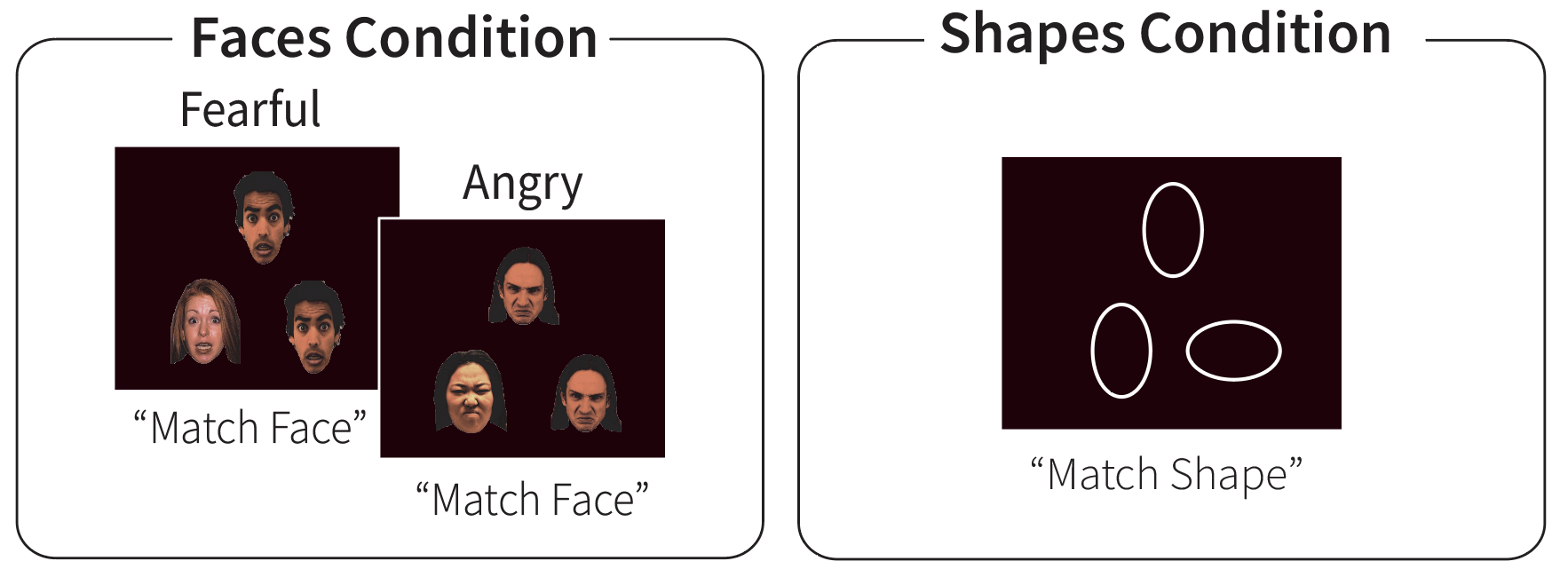
Participants are instructed to press the left button if the left-hand image on the bottom of the screen matches the top image, and to press the right button if the right-hand image on the bottom of the screen matches the top image. The bottom of the screen shows button mappings to reduce working memory demands for young children (Somerville et al., 2018).
Video Example:
Task Design:
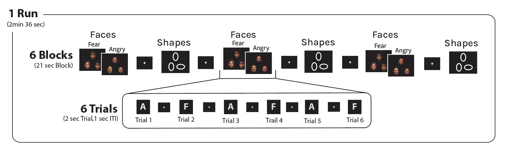
Subjects competed a single run consisting of 6 blocks (3 blocks of shape-matching and 3 blocks of face-matching). Shapes and Faces blocks are interleaved. Each block begins with a cue instructing participants to either “Match Shapes” or “Match Faces” and each block consisted of 6 trials (2 sec per trial). 3 angry and 3 fearful face trials were presented in each block. The order of the trials was randomized within each block.
Boundaries of Interest: Amygdala, Meta-Analytic ROIs, Group Average Networks

The amygdala was defined anatomically based on the Harvard-Oxford Atlas (50% threshold). The meta-analytic regions of interest (ROIs) were defined based on anatomically constrained 5mm spheres centered on meta-analytically identified peak activations (Sabatinelli et al., 2011). The Meta-Analytic ROIs included are the medial prefrontal cortex, insula, middle frontal gyrus, inferior frontal gyrus, posterior cingulate, the parietal lobule, medial temporal gyrus, and the fusiform gyrus. See below for the peak coordinates used to define the ROIs.

To evaluate group average parcellation boundaries, we used the 17 network parcellation established in Yeo et al., 2011. The parcellation approach used to establish the individualized network boundaries (detailed below) takes a global connectivity approach (Kong et al., 2019), and does not constrain based off local connectivity like some other approaches (Glasser et al., 2016; Kong et al., 2021; Schaefer et al., 2018). The Yeo 2011 parcellation most closely recapitulates the individualized approach used and thus was selected as the group average reference.
Individualized Network Parcellations
The individualized network parcellations were established using the fixation BOLD data and a parcellation pipeline developed by Kong et al., 2019, that employs a multisession hierarchical Bayesian model (MS-HBM). This model, like other clustering algorithms used to parcellate the human cortex, conceives of the cortical networks as a set of regions that exhibit similar cortico-cortical functional connectivity – i.e., all vertices within a given network will exhibit similar patterns of correlation to all other vertices in the brain (aka. have similar connectivity profiles). Here, the connectivity profile for a vertex is calculated as the Pearson’s correlation coefficient between the timeseries of the vertex and the timeseries of 1,175 regions of interest uniformly distributed across the surface (i.e. a 1 x 1,175 vector of correlation values). 1,175 ROIs are used to down sample the number of possible connections, such that the model can be estimated. Each of the 40,962 vertices on each hemisphere of the surface thus has a connectivity profile, resulting in two 40,962 x 1,175 matrices. These matrices are then binarized, retaining only the top 10% of correlations. Each of the 30 subjects will have 12 connectivity profiles matrices, one for each session. These connectivity profiles are the primary input to the multisession hierarchical Bayesian model (MS-HBM).
This model is unique in that it establishes a series of hierarchies, such that network assignment for each vertex is informed not only by a group average expectation, but also an average within-person expectation. So, though the model is initialized using network assignments from a group averaged solution obtained from an independent dataset, each individual’s parcellation is allowed to vary from that group average, as the expectation maximization estimator iterates across the levels of the hierarchy to identify an optimized solution, which results in an idiosyncratic parcellation for each subject. In the present work we used a 15-network parcellation from the HCP S900 data as the group average solution (Du et al., 2023).
A major decision during the modeling process is to select the number of networks that the model estimates. Recent work conducted by Dr. Jingnan Du and Dr. Noam Saadon-Grosman suggests a 15-network parcellation solution best recapitulates the organic connectivity visible using manual seed-based approaches on the surface (Du et al., 2023). In the 15 network-solution, a number of networks separate into two+ networks, as compared to lower-order network solutions. These separations provide better boundary fits for manual seed-based approaches than less fine gained network solutions such as a 10-network solution (used previously to parcellate the cerebellum (Xue et al., 2021). These findings suggest that a 15-network solution may be a more accurate representation of the organic systems in the brain. In lower-order network solutions such as the 10-network solution – the cingluo-opricular network, as well as the vision network are each a single large network. These two networks both segregate in the 15-network solution, the salience network/PMN breaks off from the cingluo-opricular network and the vision network separates into vision A (early visual processing areas) and B (higher order visual processing areas). Importantly, given that that we are looking at characterizing the difference in processing between visually complex, salient information (ie. threat-relevant faces) and simple non-salient information, it will be important to be able to clearly identify the salience network, as the salience network is a network that may be of note for the canonical emotion processing task. Therefore, using a 15-network solution, where these networks are clearly dissociable, will increase the specificity of the networks examined and therefore the acuity of the data/signal within the networks.
Isolating Boundary Activity:
To isolate the activity within each boundary, a similar approach to that of DiNicola, et al., 2020 was used. Activity within each boundary (amygdala, each meta-analytic ROI, each individualized network, and each group network) was extracted from the unthresholded beta maps of the Faces > Shapes contrast (‘emotion processing’ activity), as well as from the Faces > Baseline (faces condition activity) and Shapes > Baseline (shapes condition activity). Note for the boundaries in the volume (the amygdala and meta-analytic ROIs), the average activity was calculated by averaging all activity for all voxels within the ROI. For the boundaries on the surface (individualized networks and group networks), the average activity within network was then calculated by averaging all activity for all vertices within the network.
Statistical Analysis:
Project 2 and 3 were conducted using a longitudinal data set (30 subjects, each sampled 12 time). All statistical modeling was conducted within a mixed-effect framework using the lme4 package version 1.1.23 (Bates et al., 2015) in R version 4.2.1 (R Core Team, 2020), with a random effect for subject where necessary.
Project 2: Models
Boundary Activity Analysis:
We fit a separate model for activity within each of the boundary approaches and fit relative to 0 (ie. no difference in activity between the Faces and Shapes conditions).
Meta-Analytic_ROIs_Model <- lmer(Activity ~ 0 + Meta_Analytic_ROIs + (1|SubjectID), data = df) Individualized_Networks_Model <- lmer(Activity ~ 0 + Individualized_Networks + (1|SubjectID), data = df) Goup_Networks_Model <- lmer(Activity ~ 0 + Group_Networks + (1|SubjectID), data = df)
Vertex Differentiation Analysis:
For each subject’s session we fit the following model:
model <- lmer(Emotion_Processing_Activity ~ 1 + (1 | Network), data = sub_sess_data)
ICC = \(\frac{\sigma^2_\pi}{\sigma^2_\pi + \sigma^2_\epsilon}\)
Here \(\sigma^2_\pi\) is the variance of \(\pi\) (i.e., random intercept variance) and \(\sigma^2_\epsilon\) is the residual (i.e., error) variance, were extracted from the above model and used to calculate the between-network ICC value for activity within each session.
Project 3: Models
Test-retest Reliability Analysis:
For each network we fit the following model:
model <- lmer(Network ~ Session + (1 | SubjectID)), data = data)
ICC = \(\frac{\sigma^2_\pi}{\sigma^2_\pi + \sigma^2_\epsilon}\)
Here \(\sigma^2_\pi\) is the variance of \(\pi\) (i.e., random intercept variance) and \(\sigma^2_\epsilon\) is the residual (i.e., error) variance, were extracted from the above model and used to calculate the between-subject ICC value for activity within each network.
Individual Differences and Within-Subject Fluctuations Analysis:
We dissociated between and within subject components for measures of stressful life events, depression symptoms and anxiety symptoms using the following steps (Wang & Maxwell, 2015; Curren & Bauer, 2011)
- Grand mean center the variable of interest
- Compute the subject means of the centered variable (This is the between person component)
- Person mean center the variable of interest (This is the within person component)
eg. Model for examining association between early life stress and emotion processing activity within the amygdala:
Model <- Amygdala_Activity ~ Stress_Within + Stress_Between + (Stress_Within|SubjectID)